To Scale or Not to Scale

Note: If you’re looking for an article about scaling laws in AI, you might want to skip this one.

Scaling is a powerful geometric operation in shape analysis and interpenetration resolution. In shape analysis, a detailed surface often needs to be reduced to a compact description of parts and local thickness. In scene assembly, individually valid shapes may overlap, preventing their direct use in simulation. Temporarily changing geometric size can help with both tasks: it can expose redundancy in a shape representation or create room to rearrange a scene.

I will use Coverage Axis [1], its follow-up Coverage Axis++ [2], and S4R [3] to examine these two roles.

• Enlarge, then shrink. Dilating interior balls relative to a fixed surface allows coverage-based optimization to select a compact subset. Restoring the selected balls to their original radii provides a skeletal representation of the shape's principal structural features for shape analysis. [1] [2]
• Shrink, then enlarge. Shrinking objects about their initial reference centers creates clearance. Adjusting their poses as they return to full size uses this clearance to resolve interpenetration while preserving each object's shape and final dimensions. [3]

1. Scaling for Shape Abstraction

Shape analysis often requires a compact description of how a shape's parts are organized. For a chair, for example, distinguishing the broad seat from the narrow supports can matter more than preserving small surface variations. A skeletal representation captures the arrangement and thickness of parts, providing structural cues for segmentation, shape comparison, and shape recognition. [1, §1 and §9]

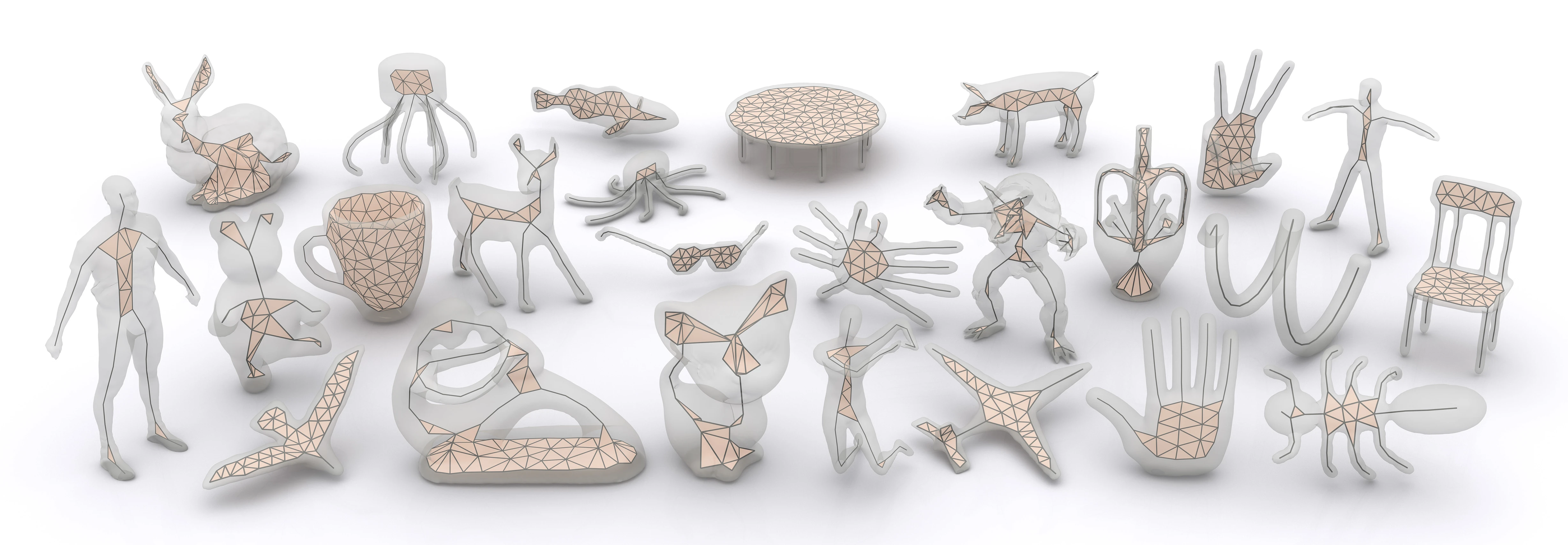
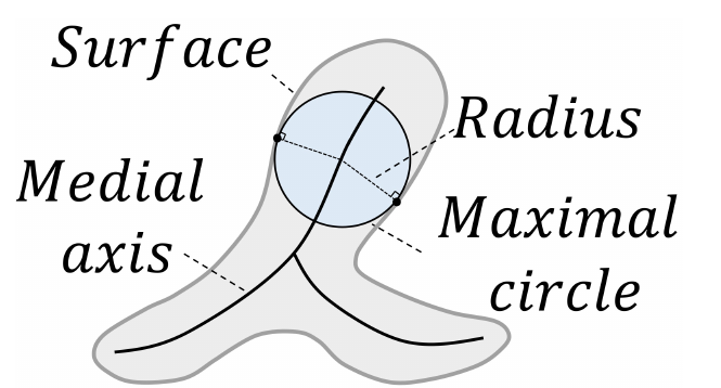
The representations in Figure 1 describe shapes through their interior structure. Their basis is Blum's medial representation: the medial axis is the locus of centers of maximal inscribed balls, and the medial axis transform (MAT) pairs those centers with their radii. [4] The centers form branches and sheets, while the radii record local thickness through distance to the boundary. In the continuous setting, the solid can be recovered as the union of its medial balls. [1, §1] Figure 2 illustrates the center–radius pairing in two dimensions.

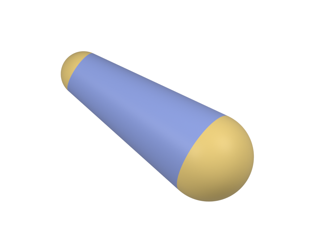
In a discrete medial mesh, the edges and triangles specify which vertex balls are interpolated together. Both center and radius vary linearly along each edge; barycentric interpolation extends the same construction across a triangle. Their continuous unions form a medial cone and a medial slab, respectively. [11, §3.1] The reconstructed shape is the union of these local volumes. Coverage Axis uses this construction for its reconstruction results. [1, §5]

Medial edge

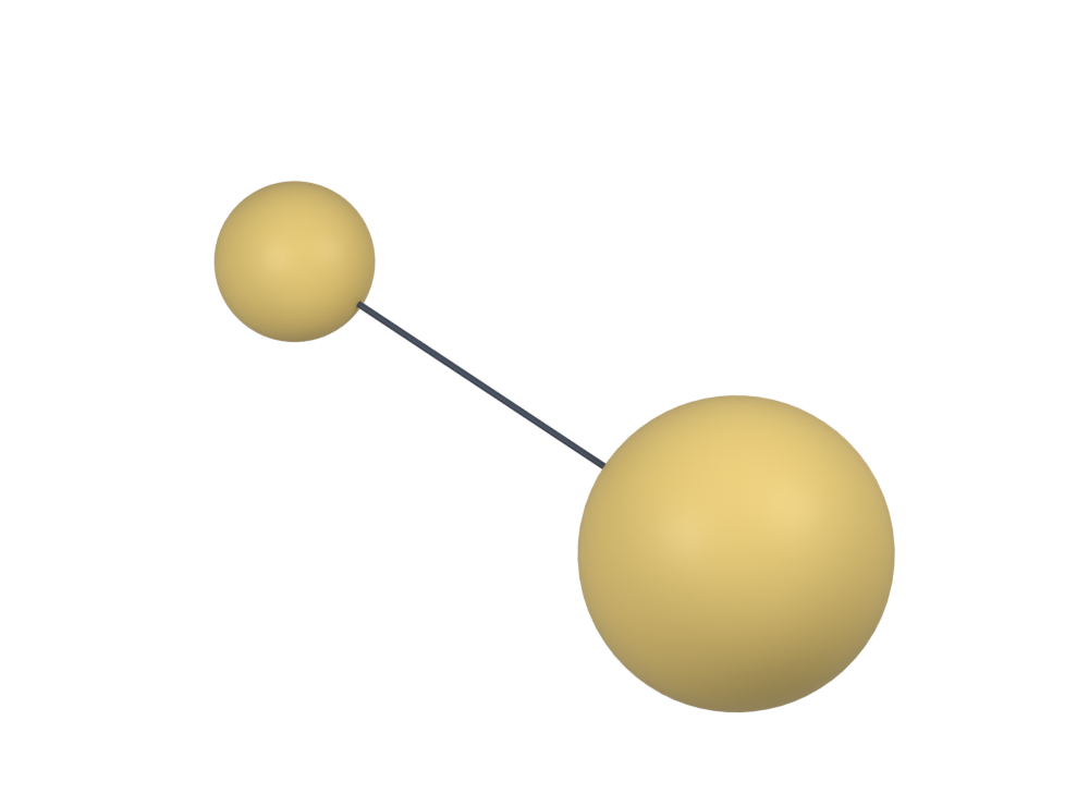
Vertex balls

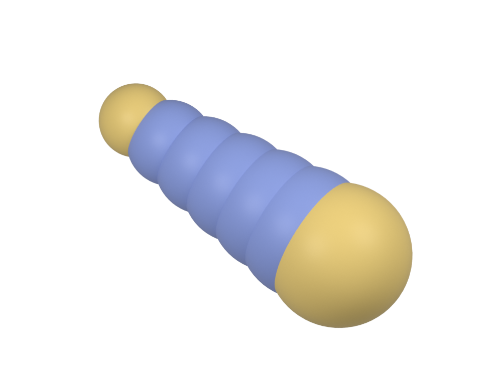
Sampled balls

Continuous envelope

Medial triangle

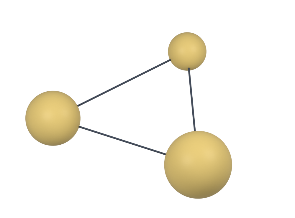
Vertex balls

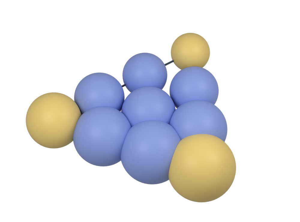
Sampled balls

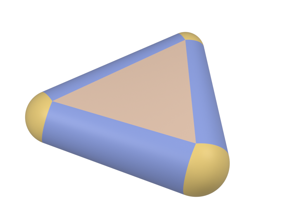
Continuous envelope

We now look at how enlarging the balls and then shrinking them back can yield a compact skeletal representation of a shape's main structural features for shape analysis.

Coverage Axis builds on a simple observation: a medial ball abstracts local geometry, while a collection of such balls can describe the whole shape. [1, §1] The task is therefore to choose the smallest collection of local descriptions that collectively accounts for the shape. This makes selection a global problem: a candidate's contribution depends on which surface regions the other selected balls can cover.

Dilation makes that collective coverage measurable. The method starts from candidate centers inside the shape, assigning each a radius estimated from its distance to the boundary; these candidates need not form an exact MAT. [1, §4.1–4.2] At its original radius, a ball may touch the surface at only a few points. Increasing that radius turns isolated contacts into patches of coverage. Overlapping patches reveal which candidates can substitute for one another, allowing the method to seek a compact set whose combined coverage accounts for every surface sample.

For a candidate center with estimated distance r_i to the boundary, the default construction adds an offset:

Each enlarged ball covers a subset of the surface samples. For n candidate centers c_i and m surface samples s_j, define the coverage matrix D(δ): its entry D_ji(δ) is 1 if ‖s_j − c_i‖₂ ≤ r_i + δ, and 0 otherwise. A binary variable v_i indicates whether candidate i is selected. Coverage Axis solves the set cover problem (SCP): [1, §4.2, Eqs. 1–2]

The objective counts the selected balls; each row of the constraint requires a surface sample to be covered at least once. For binary v, this objective has the same minimizers as the paper's ‖v‖₂ objective. A ball that accounts for a substantial local region can replace several more localized candidates; the paper relates this preference to the role of maximal inscribed balls in the MAT. [1, §1 and §6.1]

This is a point-based formulation: given the surface samples, candidate centers, and radii, the coverage matrix uses distances between points. Selection does not require the input mesh's edge or face connectivity. Once selection is complete, the retained balls use their original radii, and a separate step constructs the skeletal connectivity. [1, §4.2–4.3] The surface remains fixed throughout; dilation determines which local descriptions to keep.

This formulation explains how the offset controls the size of the representation. With the candidates, original radii, and surface samples fixed, increasing δ can only change entries of the coverage matrix from 0 to 1. Every previously feasible selection therefore remains feasible. Wherever a feasible cover exists, the optimal number of selected balls cannot increase. Their identities can still change abruptly: a continuous change in tolerance can produce a discrete change in the representation.

The reconstruction examples show what this abstraction retains. The hand keeps its finger branches, while the chair keeps a broad seat and narrow supports. The reconstructed rabbit has a smoother surface but remains recognizable through its overall form.

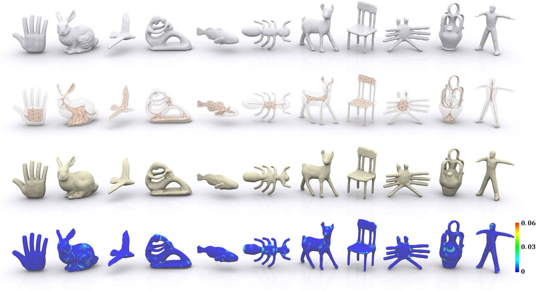
The same coverage mechanism helps explain robustness to surface noise. Dilation allows small surface variations to fall within the coverage of the same ball, so they need not introduce additional skeletal elements. The paper's noisy-surface comparisons show that the resulting compact representations retain the main shape features. [1, §6.2] Because selection operates on point sets, it also accommodates poor-quality meshes and point clouds. For point-cloud input, the paper uses surface normals to identify interior candidates before applying the same coverage formulation. [1, §4.1 and §5.2]

Tolerance and Candidate Selection

The tolerance depends on how the balls are enlarged. Adding an offset gives every ball the same absolute increase in radius; its fractional increase is δ/r_i, which is larger for smaller balls. Multiplying each radius by a common factor instead gives every ball the same relative increase. Larger balls then gain more radius in absolute terms, so the two operations treat thick and thin regions differently.

The units also matter when comparing differently sized inputs. An additive offset has units of length, so resizing an object requires resizing its offset to preserve the same coverage relationships. Normalizing the object, or expressing the offset relative to a reference length, makes that convention explicit. A multiplicative factor is dimensionless and does not require this adjustment.

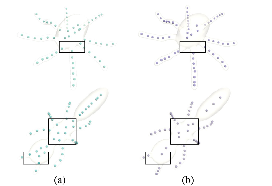
Coverage Axis compares additive and multiplicative dilation on the Octopus and Ant-3 models below. In these examples, the offset produces a more even distribution of selected points, while multiplicative scaling leaves wider gaps near junctions between parts of different thickness. The paper uses the offset by default. [1, §6.3–6.4]

The same act of enlarging balls can also serve a different construction. In the earlier Scale Axis Transform, Giesen et al. multiply medial-ball radii by a common factor, compute the MAT of their union, and divide the resulting radii by that factor. [5] That recomputation changes the medial representation itself. Coverage Axis instead keeps its candidate centers fixed and uses dilation to decide which candidates to retain.

Because selection operates on fixed candidates, their placement matters as much as the dilation rule. Moving a center changes its distance to the boundary and therefore its assigned radius and coverage patch. Changing the candidate sampling can consequently change the selected skeleton even at the same offset. The candidate set determines which structures are available to represent the shape; the selection rule determines which are retained.

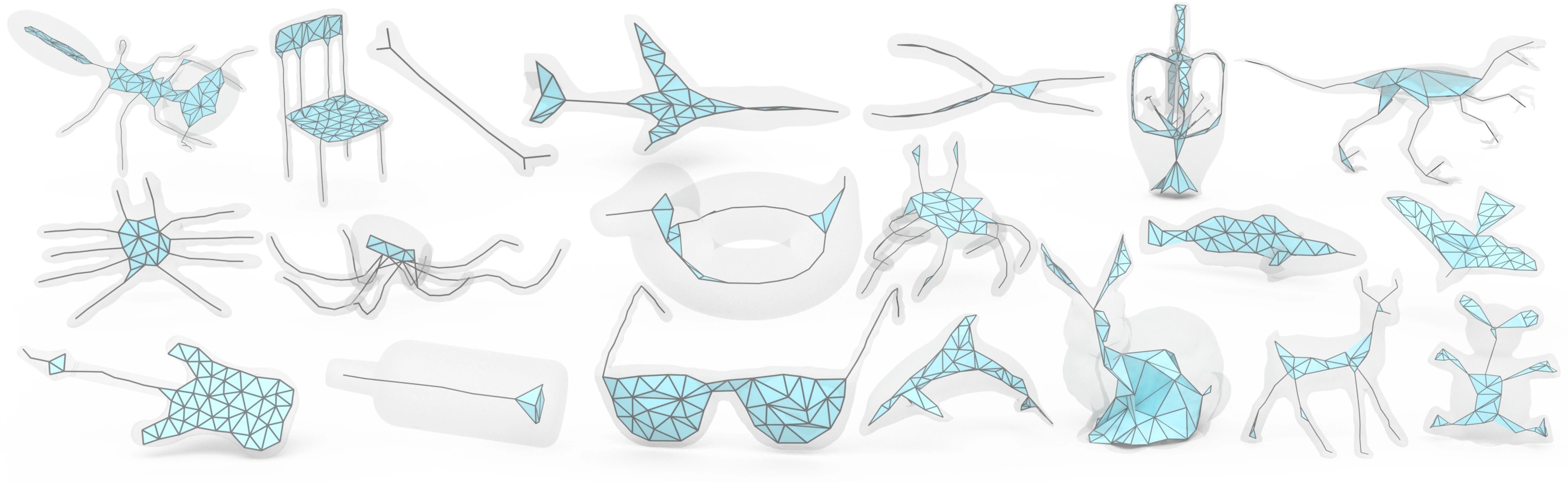
The SCP in Coverage Axis is NP-hard and can be expensive to solve. Coverage Axis++ accelerates point selection by replacing the SCP solve with an iterative heuristic. It retains the dilated-ball coverage construction and scores candidates by coverage of remaining surface samples, spatial uniformity, and centrality. [2, §1 and §4] The user specifies a point budget; selection stops when that budget is reached or all surface samples are covered. [2, §4 and §6.2]

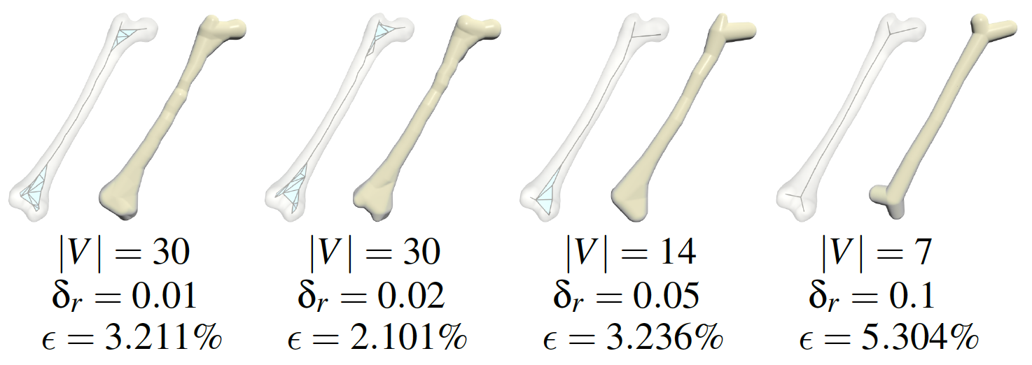
In the femur examples below, the first two offsets retain the same number of points yet yield different reconstructions; the larger offsets permit earlier termination and visibly coarsen the ends of the bone. Dilation changes which candidates can substitute for one another, while the scoring rule determines which substitutes are chosen.

2. Scaling for Resolution

Generated or independently modeled assets may each be valid shapes yet overlap when assembled. Such overlap can violate an intersection-free solver's initialization assumptions or cause large corrective motion when an impulse-based engine starts. [3, §4.7] Interpenetration resolution removes this obstacle by seeking a non-overlapping arrangement. That makes the geometry suitable for further evaluation of physical stability, graspability, and task success.

To find such an arrangement, we can first shrink the objects and then enlarge them back to full size, adjusting their poses along the way to resolve interpenetration.

S4R uses scaling to replace one deep-overlap linearization with a sequence of mostly shallow-contact quadratic programs (QPs). [3, §1] It first shrinks each body about its reference center to a small initial scale, separates centers that are too close, and verifies the resulting configuration. It then progressively restores the original dimensions while optimizing the center positions. [3, §3.2]

As the bodies grow, new contact constraints become active. At each step, a sparse QP computes the minimum-norm positional increment satisfying the active linearized constraints. By minimizing the correction at each step, S4R aims to limit layout changes as it restores full size. The default formulation updates positions; an optional variant also updates orientations. [3, §1 and §4.6]

Each intermediate configuration supplies the starting point for the next solve. This follows the strategy of numerical continuation, in which a target problem is approached through a family of related problems. [6] Geometric size defines this family; growth and positional updates jointly determine how the contact set evolves.

To isolate the effect of size on clearance, consider two spheres with fixed center distance d, original radii R₁, R₂, and a common scale factor s. Their separation margin is

While the centers stay fixed, growth reduces this margin. Once it reaches zero, further growth requires the centers to move apart to avoid penetration. For general meshes, the solver follows the same principle while updating which surface features are in contact as the bodies move.

A Quadratic Program for Each Scale Step

S4R applies this principle to triangle-mesh bodies. Bounding spheres help establish the initial small scale, and mesh queries verify the starting configuration. The default solver then keeps orientations fixed and computes a translation increment Δp_i for each body as the scale increases. [3, §3.2–3.3]

At each step, the solver predicts the separation needed to accommodate growth. For a pair of bodies, let n_ij be the unit contact direction from body i toward body j, held fixed within the current QP. Let d̃_ij^k be the detector's current score: a positive gap for separated bodies or a negative contact depth when penetration is reported.

A scale increment Δs closes the gap according to the bodies' extent along this direction. S4R bounds that closure using E_ij, the sum of their nonnegative extents from their reference centers toward one another, measured at full size in the current orientations. For a desired clearance margin d̂, the required correction along the normal is [3, §3.3.1, Eq. 3]

The active set 𝒜_k contains pairs whose predicted gap falls below the margin and for which a valid contact witness and normal are available. S4R jointly computes their positional corrections with the following convex quadratic program: [3, §3.3.3, Eq. 4]

The objective favors small translation increments across all bodies. Each constraint asks a pair's relative motion along its contact normal to make up the predicted gap deficit. Because the same body's translation appears in every contact involving it, the QP coordinates these corrections across the scene.

The solver applies the increments, advances the scale, and repeats. It periodically refreshes the mesh contacts; between full queries, cached gap predictions take the place of the measured scores. At full size, it performs further contact refinement and evaluates the returned geometry. [3, §3.4–3.5]

A useful scene may require more than separation. In the tabletop sequences below, objects must also become upright on a common support plane. This extension permits in-plane translation and yaw and restores upright orientation during growth. The objects return to their original dimensions with different positions and orientations, chosen to satisfy the additional constraints. [3, §4.8 and App. A.11]

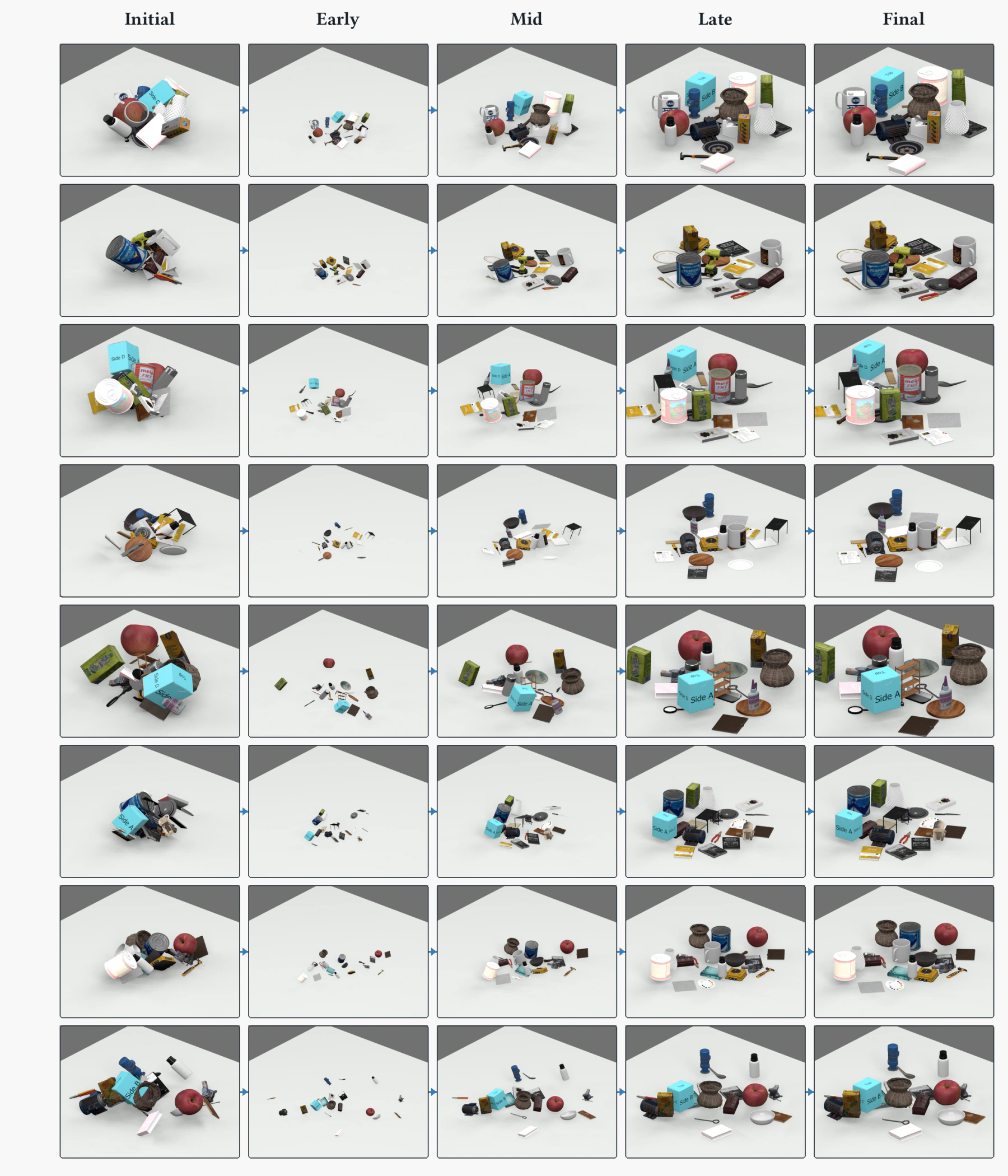
Earlier positional corrections shape later contacts, so the eventual arrangement reflects the sequence of intermediate decisions. [3, §3.3–3.5]

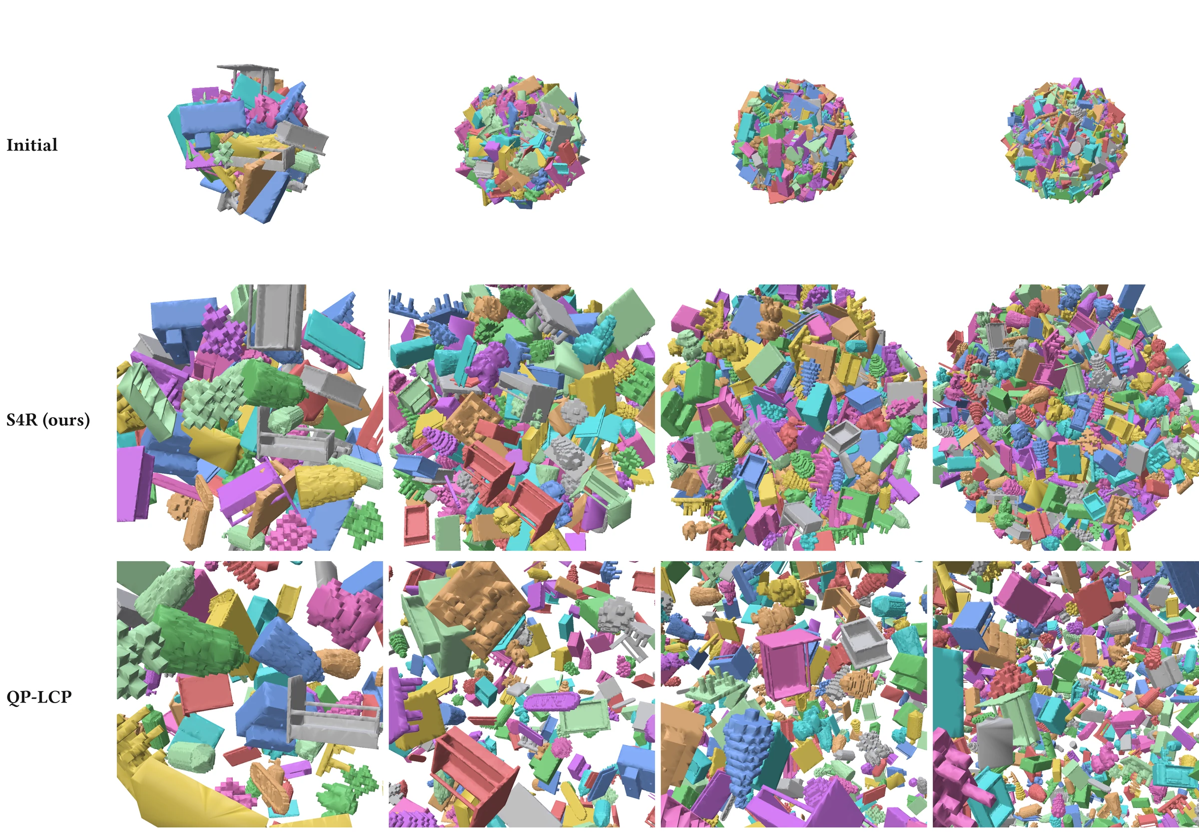
The dense-scene comparison below makes the resulting spatial organization visible. S4R and a QP/LCP baseline begin from the same crowded configurations and reach different distributions of bodies. Viewing each pair from the same camera shows how their correction strategies affect the spread of the full-size scene. [3, App. A.13]

3. What Scaling Leaves Behind

These examples reveal two distinct roles for scale. In Coverage Axis, a chosen tolerance defines which candidates can cover each surface sample. Solving at several offsets gives a family of representations, but each selection problem can be solved independently. S4R instead uses intermediate scales within a single computation, carrying a configuration forward until the prescribed dimensions are restored. The first parameter sets a coverage tolerance; the second controls how the solver approaches the target geometry.

In both cases, restoring dimensions leaves a computational decision in place. The selected balls keep their identities when their original radii are restored, so the coverage tolerance continues to determine the skeletal representation. Likewise, restoring an object's size preserves the positional changes accumulated during resolution. This is why a temporary change in size can have a lasting effect on the result.

4. From Scene Editing to Manipulation

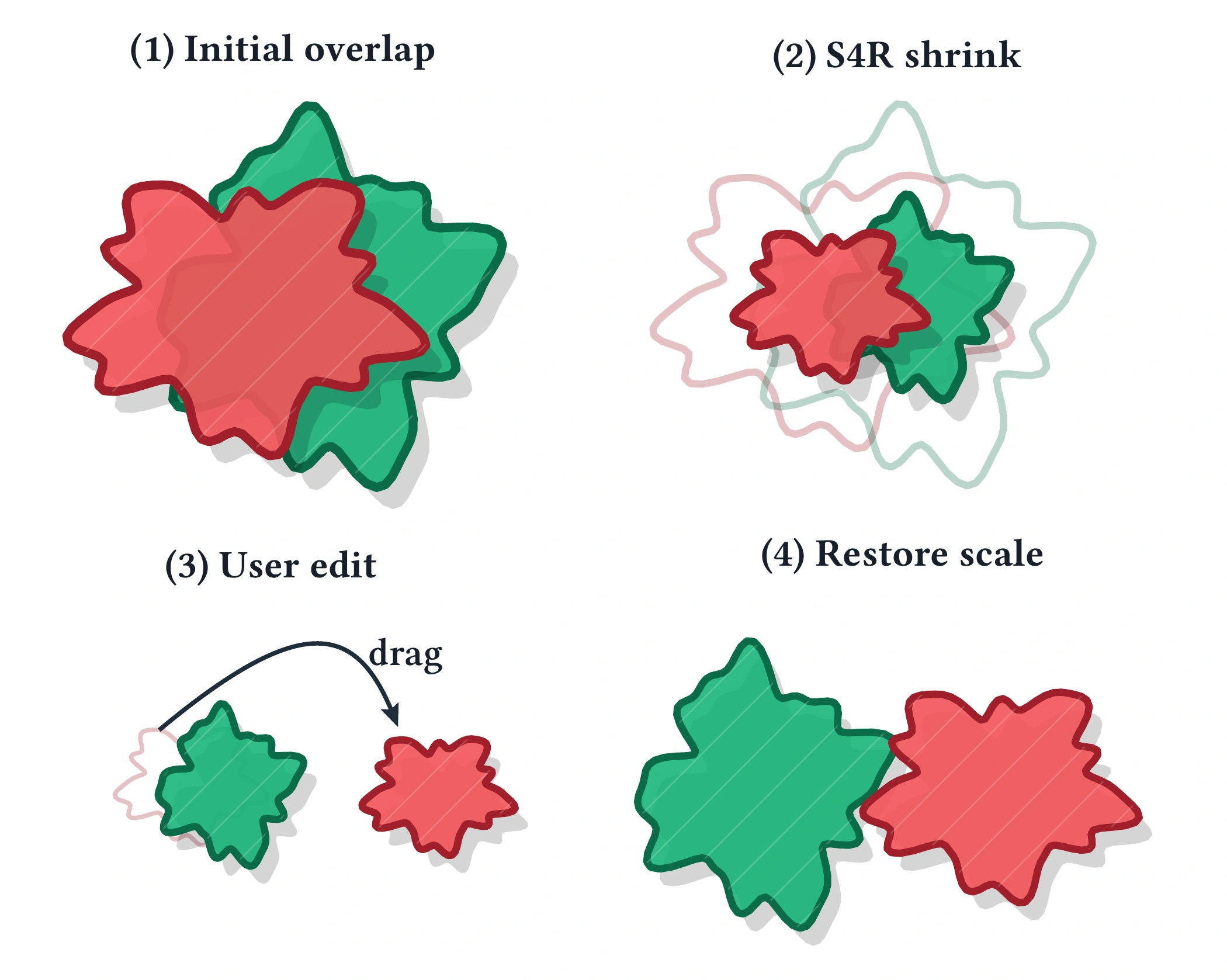
Because intermediate placements influence the restored layout, they also offer a way to specify layout intent. S4R's editable scale-space example demonstrates a user moving shrunken objects before restoring their dimensions. [3, Fig. 9] An agent could act at the same stage, translating a request into relative placements and constraints for the geometric solver to enforce during restoration. Relations such as left-of remain meaningful even while object sizes change.

Language-Guided Scene Layout

An implementation of this interface is SimReady_Gate. In its twenty-object example, RoboLab catalog objects begin in a heap, with their reference centers sampled within a disk of radius 13 cm and 82 object–object interpenetrating pairs. The request asks for a cooking layout: the bowl in front of the pitcher, the ladle and spoon within reach, fruit grouped on the left, cans and bottles along the back, and the hammer, bin, remote, and spatula on the right. A language-derived program supplies placements for the shrunken objects and constraints for their restoration. [8]

The recorded loop takes two rounds because the initial program adds an exact coordinate target for the hammer, although the request only specifies its placement on the right. The first repair removes the intersections but misses that coordinate target. The agent then removes the extra constraint while retaining the requested right-of relation. The successful repair and geometric checks take about 30 seconds, returning a full-size layout with zero interpenetrating pairs reported by the mesh verifier and all 97 implemented predicates satisfied at their specified tolerances. [8] The revision illustrates a useful role for an agent: identifying when a failure comes from an overly restrictive translation of the request into a program.

Manipulation in Repaired Scenes

The next demonstration places repair and physical settling before a manipulation task. S4R first resolves interpenetrations in a scene of 48 YCB objects, which is then settled in simulation. A simulated Franka arm subsequently picks up the sugar box and places it inside a ring. [9]

1. S4R repair and settling (0:00) 2. Franka pick and place (0:13)

5. Future Directions

These ideas suggest several next steps: preserve the shape features a task needs, choose when and how fast objects grow back, and account for how a repaired scene behaves in simulation.

Choosing Which Shape Features to Keep

Larger dilation lets fewer balls cover the surface, but can also remove small structures. For grasping, the shape of a handle matters more than surface decoration. We could therefore use stricter coverage tolerances around the handle and allow more simplification elsewhere.

Coverage Axis already allows some surface samples to be left out of the coverage requirement. [1, §7.2] Giving different regions different tolerances would offer finer control, but the rule must apply to every ball that could cover that region. Reducing dilation only for balls near the handle would not be enough: a large ball centered elsewhere could still cover its samples, causing the selection to discard the balls that describe the handle.

A different primitive may help with parts that balls represent inefficiently. A chair seat, for example, is wide and thin, so it may take many balls to describe. Future work could therefore explore alternatives, including ellipsoids, which can be wide in one direction and thin in another. [2, §6.6] Ellipsoidal bounding volumes have already been studied in shape decomposition. [7]

Lengthening an ellipsoid's three axes by the same amount does not generally move its whole surface outward by a constant distance. To use ellipsoids here, we would need to define how their dilation controls coverage and how the selected set reconstructs the shape.

Choosing How Objects Return to Full Size

The way objects grow back affects their final positions. Minimizing each position adjustment does not guarantee the smallest final displacement. Objects can also get stuck in a confined space even when a different arrangement would fit at full size. Each local QP is convex, but the full layout problem remains nonconvex. [3, §3.3.3 and §5]

Even a small increase in size can require a large movement. After that movement, different surface features may be closest, so the previous contact approximation may no longer be accurate. S4R updates contacts during growth and checks and refines the layout at full size. [3, §3.3–3.5] In the larger scenes in Figure 10, the default refinement budget leaves some overlaps; additional refinement removes them in these examples. [3, App. A.13]

One possibility is to choose a separate growth schedule for each object. If one object blocks another, we could pause its growth while moving the other into place. The solver would need to update contacts as they move and eventually restore every object to its original size. Future work could also explore jumping over a range of scales with no feasible intermediate solution. [3, §5]

From Geometric Repair to Physical Interaction

Removing overlaps does not ensure that objects will stay where we want them. In the twenty-object example, the repaired layout passes its geometric checks, but some round fruit lose their required upright orientation during MuJoCo settling. [8] An agent needs to distinguish failures caused by overlap, unmet spatial relationships, and behavior in simulation.

For scenes that will be simulated, a next step would be to account for mass, friction, and velocity during repair, so that the initial conditions also reflect how the objects will move. [3, §5]

Virtual dressing introduces further challenges: body motion, cloth deformation, and the passage of limbs through garment openings must be coordinated. [10] Simply shrinking a human mesh, placing it inside a garment, and restoring its size would not ensure a correctly dressed configuration. S4R does not currently handle these interactions.

For a pullover, each arm must enter the correct sleeve and the neck must pass through the neck opening. Any such extension would have to establish this arrangement and keep it as the body grows, while preventing body–cloth penetration and self-intersection. Even if this produces a correctly dressed configuration, finding a physical dressing motion that reaches it would remain a separate planning problem.

References

1. Zhiyang Dou, Cheng Lin, Rui Xu, Lei Yang, Shiqing Xin, Taku Komura, and Wenping Wang. 2022. Coverage Axis: Inner Point Selection for 3D Shape Skeletonization. Computer Graphics Forum 41, 2, 419–432.
2. Zimeng Wang, Zhiyang Dou, Rui Xu, Cheng Lin, Yuan Liu, Xiaoxiao Long, Shiqing Xin, Taku Komura, Xiaoming Yuan, and Wenping Wang. 2024. Coverage Axis++: Efficient Inner Point Selection for 3D Shape Skeletonization. Computer Graphics Forum 43, 5, e15143. DOI.
3. Zhiyang Dou, Ang Zhao, Chen Peng, Minghao Guo, Haixu Wu, Cheng Lin, Yuan Liu, Junfeng Yao, Xiaohu Guo, Wenping Wang, and Wojciech Matusik. 2026. S4R: Scaling for Rigid-Body Interpenetration Resolution. ACM Transactions on Graphics 45, 6, Article 197. DOI.
4. Harry Blum. 1967. A Transformation for Extracting New Descriptors of Shape. In Models for the Perception of Speech and Visual Form, Weiant Wathen-Dunn (ed.). MIT Press, 362–380.
5. Joachim Giesen, Balint Miklos, Mark Pauly, and Camille Wormser. 2009. The Scale Axis Transform. In Proceedings of the Twenty-Fifth Annual Symposium on Computational Geometry, 106–115.
6. Eugene L. Allgower and Kurt Georg. 2003. Introduction to Numerical Continuation Methods. Classics in Applied Mathematics, Vol. 45. Society for Industrial and Applied Mathematics.
7. Lin Lu, Yi-King Choi, Wenping Wang, and Myung-Soo Kim. 2007. Variational 3D Shape Segmentation for Bounding Volume Computation. Computer Graphics Forum 26, 3, 329–338.
8. Zhiyang Dou. 2026. SimReady_Gate. Research software, README and recorded twenty-object example, commit 91cbaf2. Accessed 20 September 2026. Repair log · Constraint log · Final certificate.
9. Zhiyang Dou. 2026. S4R code and simulated manipulation demonstration. Research software and recorded demonstration, commit 91cbaf2. Accessed 20 September 2026. Repair and settle video · Pick and place video.
10. Alexander Clegg, Jie Tan, Greg Turk, and C. Karen Liu. 2015. Animating Human Dressing. ACM Transactions on Graphics 34, 4, Article 116, 1–9. Paper.
11. Pan Li, Bin Wang, Feng Sun, Xiaohu Guo, Caiming Zhang, and Wenping Wang. 2015. Q-MAT: Computing Medial Axis Transform By Quadratic Error Minimization. ACM Transactions on Graphics 35, 1, Article 8, 1–16. DOI.

@misc{dou2026toscale,
  author = {Dou, Zhiyang},
  title = {To Scale or Not to Scale},
  year = {2026},
  month = sep,
  howpublished = {Research Notes},
  url = {https://frank-zy-dou.github.io/blog/to-scale-or-not-to-scale/}
}